1.基本概念的描述
1.1为什么做数据分析
了解我们要研究的对象的基本情况,探讨变量间的相互关系
抽样分析。如果能够获得总体的数据,那么“数据即是理论”,而不需要进行推断统计
由“科学”到“广义科学”:从寻求确定的结果到寻求稳定区间内的结果
1.2总体与样本
总体(population):全体CSNU的学生
样本(sample):CSNU心理学专业学生
总体参数:CSNU平均学习时间
样本统计量:CSNU心理学专业学生的平均学习时间
样本统计量 ≠ 总体参数
因此,从样本推论总体情况的时候,总是存在(不准确的情况)误差
置信区间(confidence interval):有多大的概率我们估计的数据会落入这一区间内
1.3数据类型
- 定性数据
- 称名数据:性别,专业等
- 顺序数据:学历
- 定量数据
- 离散数据:学生人数(只能计为个数,不存在小数)
- 连续数据:体重,年龄等
1.4显著性水平与统计功效
显著性水平:犯第一类错误的最大概率的大小α。
p值:当H0是对的时,然后给定某个数,跟这个数一样极端或者比它还极端的概率就是P-value。
统计功效:统计功效指的是在假设检验中,H1(alternative hypothesis)为真时,正确地拒绝H0(null hypothesis)的概率,或者1-β。
一类错误与二类错误:
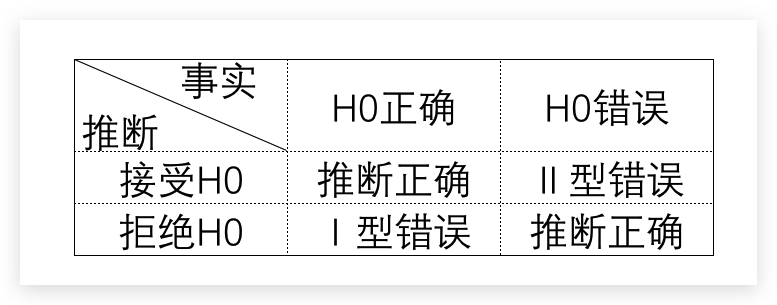
1.4显著性水平与统计功效
- 举例:在未来,女性已经统治了地球,他们觉的男人太过讨厌,于是想了一个办法来清除男性,他们商讨一番,决定使用的新鲜武器:自动判别,如果小于A罩杯,则杀无赦;如果等于或大于A罩杯,则放过。这个武器本意是区分男性和女性,杀死所有男性,放过所有女性。硝烟过后,大家可以想象得到结果,有些可怜的mm因为胸太小被误杀,这就是武器的判别程序犯的一类错误。本属于女性这个群体,却被错误的判断为不属于。有些胸肌发达的gg因为胸很大而活下来,这就是武器的判别程序犯的二类错误,本不属于女性这个群体,却被误判为属于。而所有被杀害的男性,则是该判别程序的效力(power,i.e. 1-β)。
1.5信度与效度
- 信度:问卷或测量工具的稳定性指标,说明可重复性的可能
效度:针对某一变量的问卷或测量工具有效性程度。
效度高,信度一定高;信度高,效度不一定高。
2.描述性统计
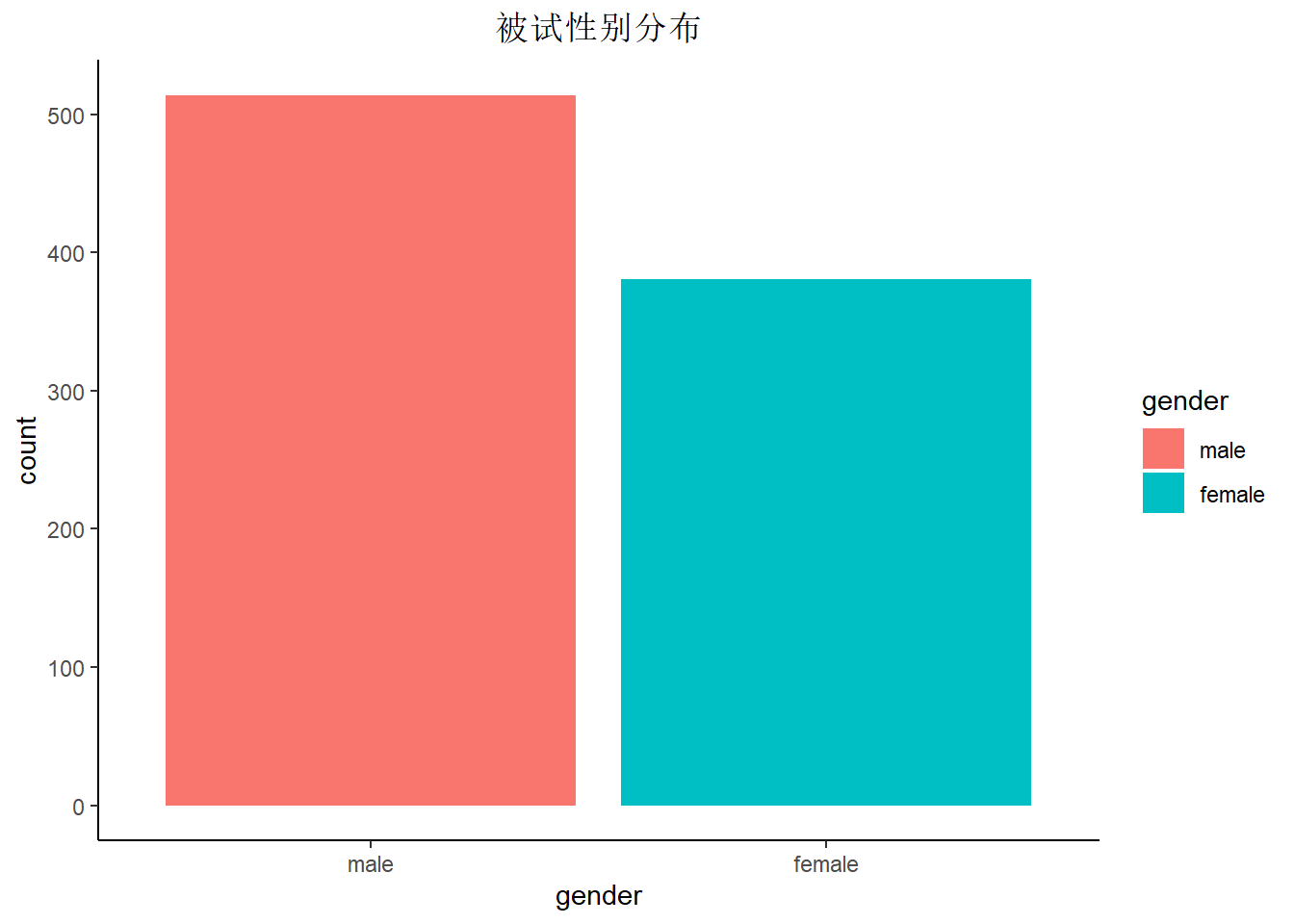
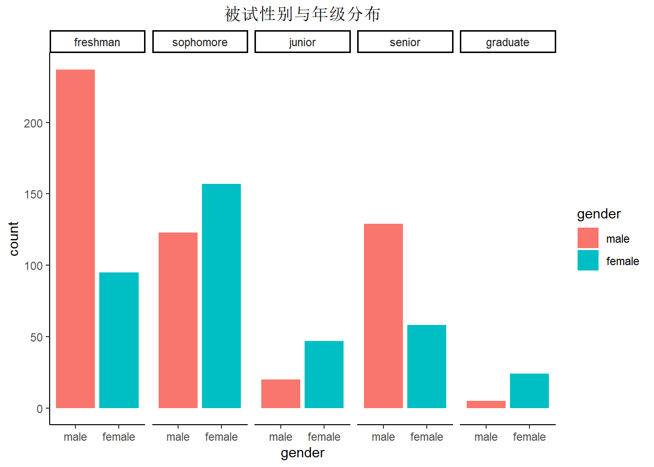
2.1 被试群体的基本信息
- 举例:大学生社会流动信念是如何影响学习投入的?
- 被试性别分布
- 被试性别与年级分布
2.2研究工具的信、效度
- 信度分析
##
## 载入程辑包:'psych'
## The following objects are masked from 'package:ggplot2':
##
## %+%, alpha## [1] 0.8586419## [1] 0.8925558## [1] 0.9360799## [1] 0.9561618- 效度分析:以社会阶层流动信念问卷为例
## This is lavaan 0.6-3## lavaan is BETA software! Please report any bugs.##
## 载入程辑包:'lavaan'## The following object is masked from 'package:psych':
##
## cor2cov## lavaan 0.6-3 ended normally after 22 iterations
##
## Optimization method NLMINB
## Number of free parameters 12
##
## Number of observations 895
##
## Estimator ML
## Model Fit Test Statistic 287.879
## Degrees of freedom 9
## P-value (Chi-square) 0.000
##
## Model test baseline model:
##
## Minimum Function Test Statistic 2454.614
## Degrees of freedom 15
## P-value 0.000
##
## User model versus baseline model:
##
## Comparative Fit Index (CFI) 0.886
## Tucker-Lewis Index (TLI) 0.809
##
## Loglikelihood and Information Criteria:
##
## Loglikelihood user model (H0) -7682.579
## Loglikelihood unrestricted model (H1) -7538.639
##
## Number of free parameters 12
## Akaike (AIC) 15389.157
## Bayesian (BIC) 15446.719
## Sample-size adjusted Bayesian (BIC) 15408.609
##
## Root Mean Square Error of Approximation:
##
## RMSEA 0.186
## 90 Percent Confidence Interval 0.168 0.205
## P-value RMSEA <= 0.05 0.000
##
## Standardized Root Mean Square Residual:
##
## SRMR 0.068
##
## Parameter Estimates:
##
## Information Expected
## Information saturated (h1) model Structured
## Standard Errors Standard
##
## Latent Variables:
## Estimate Std.Err z-value P(>|z|) Std.lv Std.all
## G =~
## a1 1.000 0.836 0.691
## a2 1.116 0.056 19.897 0.000 0.933 0.746
## a3 0.957 0.061 15.663 0.000 0.800 0.575
## a4 1.174 0.054 21.799 0.000 0.982 0.834
## a5 0.855 0.050 17.177 0.000 0.715 0.634
## a6 1.210 0.058 20.805 0.000 1.012 0.786
##
## Variances:
## Estimate Std.Err z-value P(>|z|) Std.lv Std.all
## .a1 0.764 0.041 18.424 0.000 0.764 0.522
## .a2 0.694 0.040 17.379 0.000 0.694 0.444
## .a3 1.298 0.066 19.698 0.000 1.298 0.670
## .a4 0.421 0.030 14.231 0.000 0.421 0.304
## .a5 0.760 0.040 19.157 0.000 0.760 0.598
## .a6 0.634 0.039 16.258 0.000 0.634 0.382
## G 0.699 0.062 11.201 0.000 1.000 1.000
##
## R-Square:
## Estimate
## a1 0.478
## a2 0.556
## a3 0.330
## a4 0.696
## a5 0.402
## a6 0.618- 效度分析:以学习投入量表为例
## lavaan 0.6-3 ended normally after 51 iterations
##
##   Optimization method                           NLMINB
##   Number of free parameters                         37
##
##   Number of observations                           895
##
##   Estimator                                         ML
##   Model Fit Test Statistic                    1731.394
##   Degrees of freedom                               116
##   P-value (Chi-square)                           0.000
##
## Model test baseline model:
##
##   Minimum Function Test Statistic            12656.568
##   Degrees of freedom                               136
##   P-value                                        0.000
##
## User model versus baseline model:
##
##   Comparative Fit Index (CFI)                    0.871
##   Tucker-Lewis Index (TLI)                       0.849
##
## Loglikelihood and Information Criteria:
##
##   Loglikelihood user model (H0)             -20293.204
##   Loglikelihood unrestricted model (H1)     -19427.507
##
##   Number of free parameters                         37
##   Akaike (AIC)                               40660.409
##   Bayesian (BIC)                             40837.891
##   Sample-size adjusted Bayesian (BIC)        40720.386
##
## Root Mean Square Error of Approximation:
##
##   RMSEA                                          0.125
##   90 Percent Confidence Interval          0.120  0.130
##   P-value RMSEA <= 0.05                          0.000
##
## Standardized Root Mean Square Residual:
##
##   SRMR                                           0.061
##
## Parameter Estimates:
##
##   Information                                 Expected
##   Information saturated (h1) model          Structured
##   Standard Errors                             Standard
##
## Latent Variables:
##                    Estimate  Std.Err  z-value  P(>|z|)   Std.lv  Std.all
##   f1 =~
##     d1                1.000                               0.882    0.603
##     d2                1.018    0.059   17.229    0.000    0.899    0.681
##     d3                1.133    0.062   18.401    0.000    1.000    0.746
##     d5                0.974    0.053   18.372    0.000    0.859    0.745
##     d7                1.297    0.062   20.757    0.000    1.144    0.895
##     d9                1.216    0.063   19.290    0.000    1.073    0.799
##   f2 =~
##     d4                1.000                               0.958    0.759
##     d8                1.141    0.039   29.462    0.000    1.094    0.884
##     d10               1.180    0.041   29.023    0.000    1.131    0.873
##     d12               1.034    0.044   23.439    0.000    0.991    0.731
##     d15               0.976    0.041   24.060    0.000    0.935    0.748
##     d17               0.970    0.056   17.177    0.000    0.930    0.554
##   f3 =~
##     d6                1.000                               0.954    0.781
##     d11               1.190    0.039   30.652    0.000    1.135    0.873
##     d13               1.021    0.042   24.506    0.000    0.974    0.735
##     d14               0.725    0.038   19.315    0.000    0.691    0.602
##     d16               0.952    0.048   19.782    0.000    0.908    0.615
##
## Covariances:
##                    Estimate  Std.Err  z-value  P(>|z|)   Std.lv  Std.all
##   f1 ~~
##     f2                0.854    0.061   14.033    0.000    1.011    1.011
##   f2 ~~
##     f3                0.948    0.058   16.446    0.000    1.038    1.038
##   f1 ~~
##     f3                0.847    0.060   14.181    0.000    1.007    1.007
##
## Variances:
##                    Estimate  Std.Err  z-value  P(>|z|)   Std.lv  Std.all
##    .d1                1.366    0.066   20.717    0.000    1.366    0.637
##    .d2                0.933    0.046   20.475    0.000    0.933    0.536
##    .d3                0.795    0.039   20.140    0.000    0.795    0.443
##    .d5                0.593    0.029   20.152    0.000    0.593    0.445
##    .d7                0.324    0.019   17.207    0.000    0.324    0.198
##    .d9                0.651    0.033   19.675    0.000    0.651    0.361
##    .d4                0.677    0.033   20.655    0.000    0.677    0.425
##    .d8                0.335    0.017   19.236    0.000    0.335    0.219
##    .d10               0.398    0.020   19.509    0.000    0.398    0.237
##    .d12               0.855    0.041   20.750    0.000    0.855    0.465
##    .d15               0.690    0.033   20.696    0.000    0.690    0.441
##    .d17               1.951    0.093   21.023    0.000    1.951    0.693
##    .d6                0.581    0.028   20.460    0.000    0.581    0.390
##    .d11               0.404    0.022   18.656    0.000    0.404    0.239
##    .d13               0.807    0.039   20.753    0.000    0.807    0.460
##    .d14               0.840    0.040   21.057    0.000    0.840    0.638
##    .d16               1.358    0.065   21.043    0.000    1.358    0.622
##     f1                0.779    0.079    9.821    0.000    1.000    1.000
##     f2                0.918    0.069   13.372    0.000    1.000    1.000
##     f3                0.910    0.065   13.930    0.000    1.000    1.000
##
## R-Square:
##                    Estimate
##     d1                0.363
##     d2                0.464
##     d3                0.557
##     d5                0.555
##     d7                0.802
##     d9                0.639
##     d4                0.575
##     d8                0.781
##     d10               0.763
##     d12               0.535
##     d15               0.559
##     d17               0.307
##     d6                0.610
##     d11               0.761
##     d13               0.540
##     d14               0.362
##     d16               0.378
2.3 描述统计
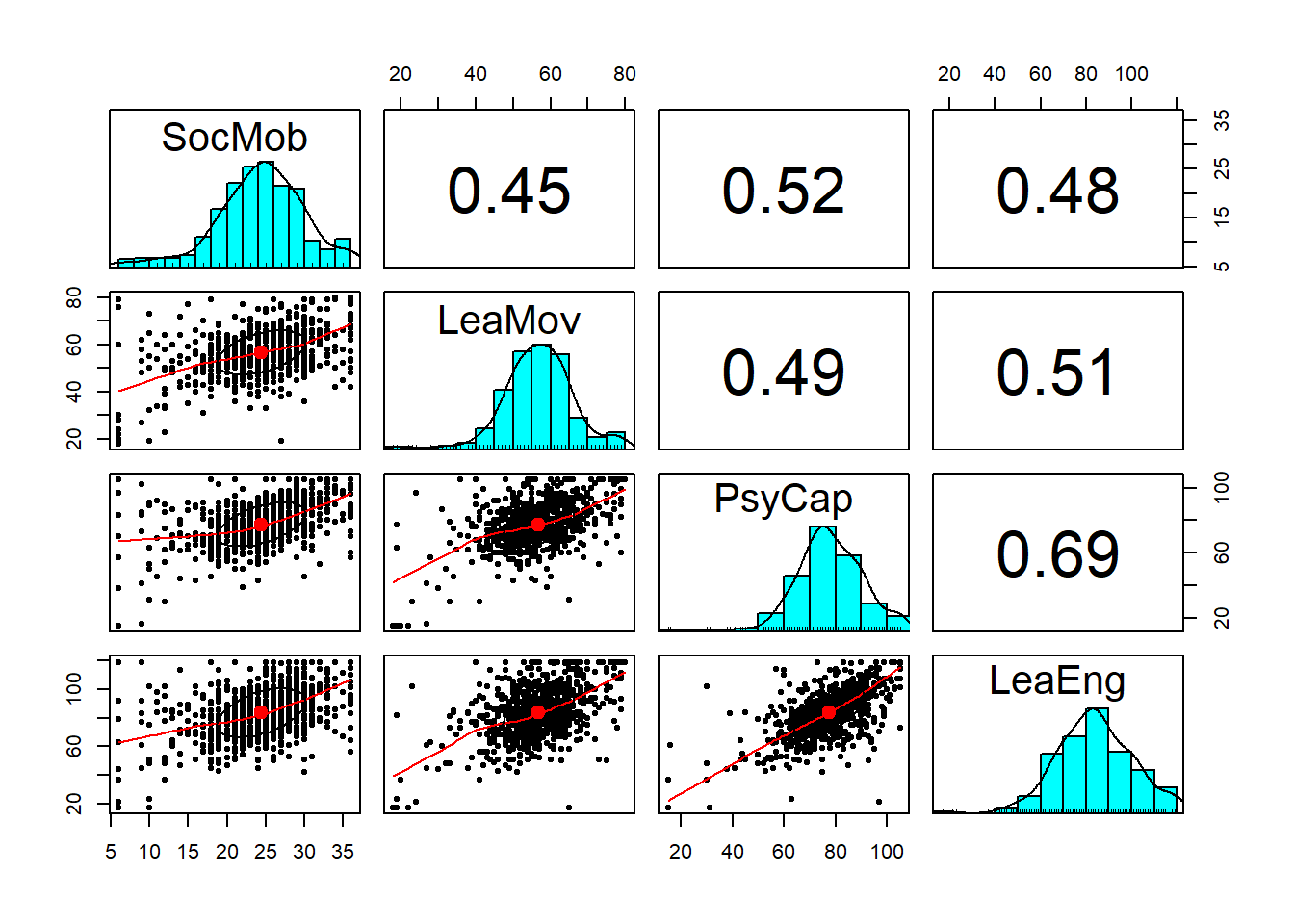
- 平均数M:用于描述群体基本状况的数据
- 标准差SD:用于描述群体数据离散程度的数据,标准差越大,群体数据越分散。
##        vars   n  mean    sd median trimmed   mad min max range  skew
## SocMob    1 895 24.42  5.69     25   24.63  4.45   6  36    30 -0.50
## LeaMov    2 895 56.81  9.45     57   56.95  8.90  18  80    62 -0.47
## PsyCap    3 895 77.57 13.60     77   77.84 11.86  15 105    90 -0.70
## LeaEng    4 895 83.76 17.15     84   83.87 16.31  17 119   102 -0.30
##        kurtosis   se
## SocMob     0.86 0.19
## LeaMov     1.92 0.32
## PsyCap     2.64 0.45
## LeaEng 0.90 0.57- 相关系数r: 用于描述两个变量之间的关系
2.4推断统计
- t检验:用于描述变量在两个水平上差异的检验方法。
- 社会流动信念t检验
## 载入需要的程辑包:boot##
## 载入程辑包:'boot'## The following object is masked from 'package:psych':
##
## logit## 载入需要的程辑包:magrittr## DABEST (Data Analysis with Bootstrap Estimation) v0.2.2
## =======================================================
##
## Variable: SocMob
##
## Unpaired mean difference of female (n=514) minus male (n=381)
## -0.0917 [95CI -0.838; 0.602]
##
##
## 5000 bootstrap resamples.
## All confidence intervals are bias-corrected and accelerated.
- 学习动机t检验
## DABEST (Data Analysis with Bootstrap Estimation) v0.2.2
## =======================================================
##
## Variable: LeaMov
##
## Unpaired mean difference of female (n=514) minus male (n=381)
##  -1.35 [95CI  -2.55; -0.142]
##
##
## 5000 bootstrap resamples.
## All confidence intervals are bias-corrected and accelerated.
- ANOVA检验:在描述性统计部分,主要了解单因素方差分析
3.中介作用
3.1概念模型
##
## 载入程辑包:'processR'
## The following object is masked from 'package:psych':
##
## corPlot
3.2统计模型
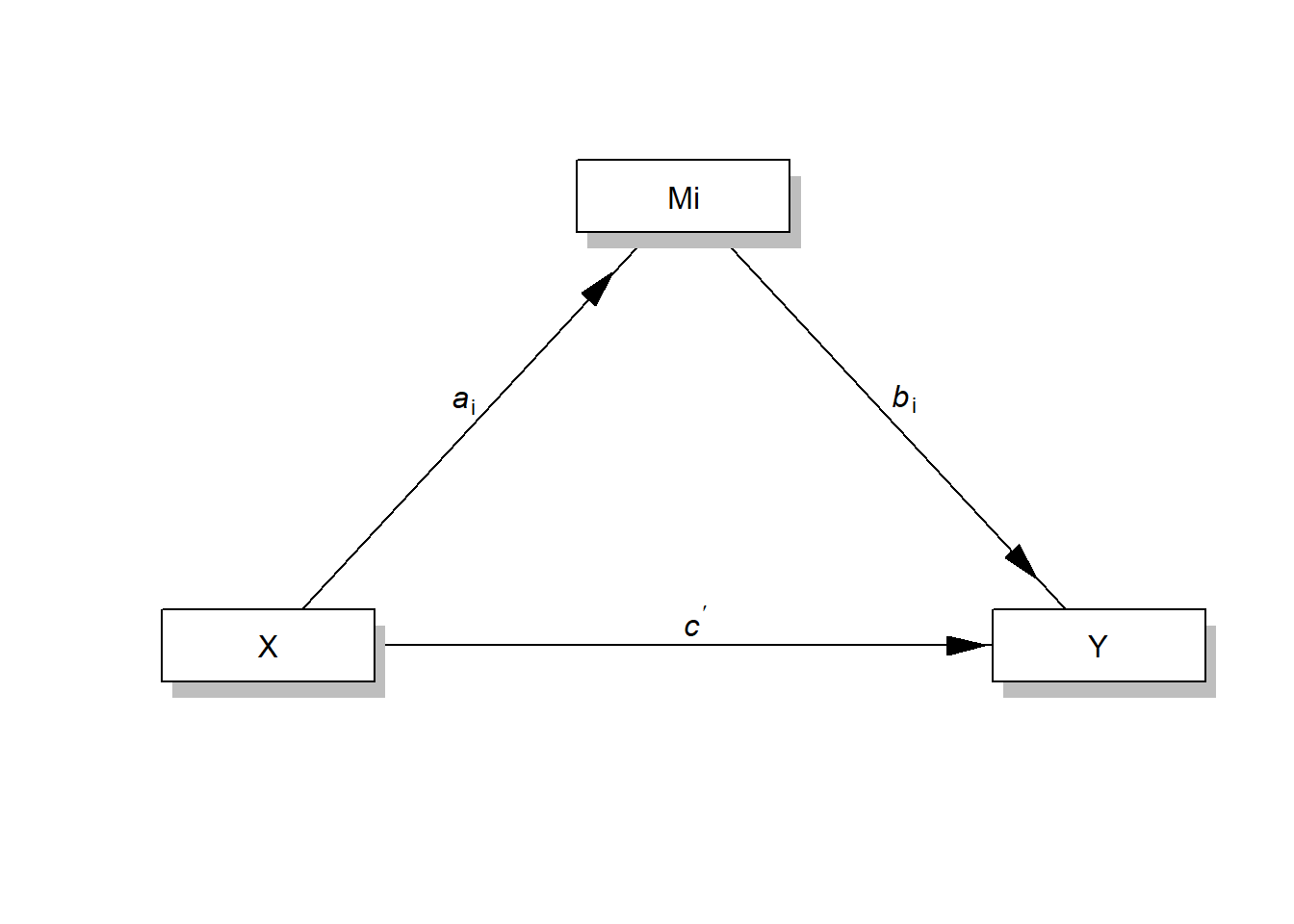
3.3中介模型的实现
## LeaMov~a*SocMob
## LeaEng~c*SocMob+b*LeaMov
## indirect :=(a)*(b)
## direct :=c
## total := direct + indirect
## prop.mediated := indirect / total
## lavaan 0.6-3 ended normally after 19 iterations
##
## Optimization method NLMINB
## Number of free parameters 5
##
## Number of observations 895
##
## Estimator ML
## Model Fit Test Statistic 0.000
## Degrees of freedom 0
## Minimum Function Value 0.0000000000000
##
## Parameter Estimates:
##
## Information Expected
## Information saturated (h1) model Structured
## Standard Errors Standard
##
## Regressions:
## Estimate Std.Err z-value P(>|z|)
## LeaMov ~
## SocMob (a) 0.752 0.049 15.199 0.000
## LeaEng ~
## SocMob (c) 0.950 0.092 10.379 0.000
## LeaMov (b) 0.673 0.055 12.213 0.000
##
## Variances:
## Estimate Std.Err z-value P(>|z|)
## .LeaMov 70.906 3.352 21.154 0.000
## .LeaEng 192.941 9.121 21.154 0.000
##
## Defined Parameters:
## Estimate Std.Err z-value P(>|z|)
## indirect 0.506 0.053 9.520 0.000
## direct 0.950 0.092 10.379 0.000
## total 1.456 0.088 16.523 0.000
## prop.mediated 0.348 0.038 9.251 0.0004.调节作用
4.1概念模型
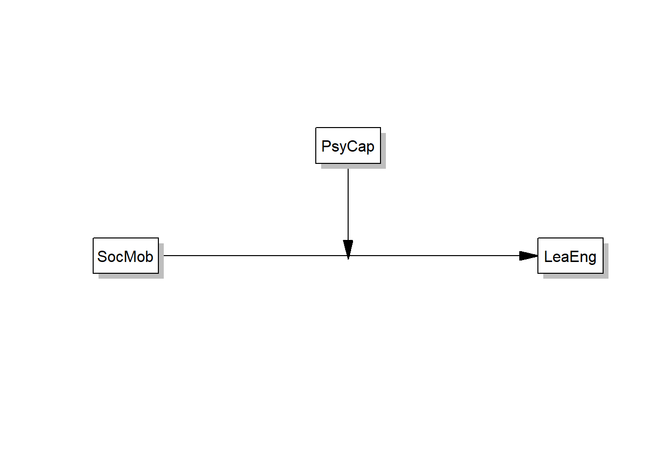
4.2统计模型
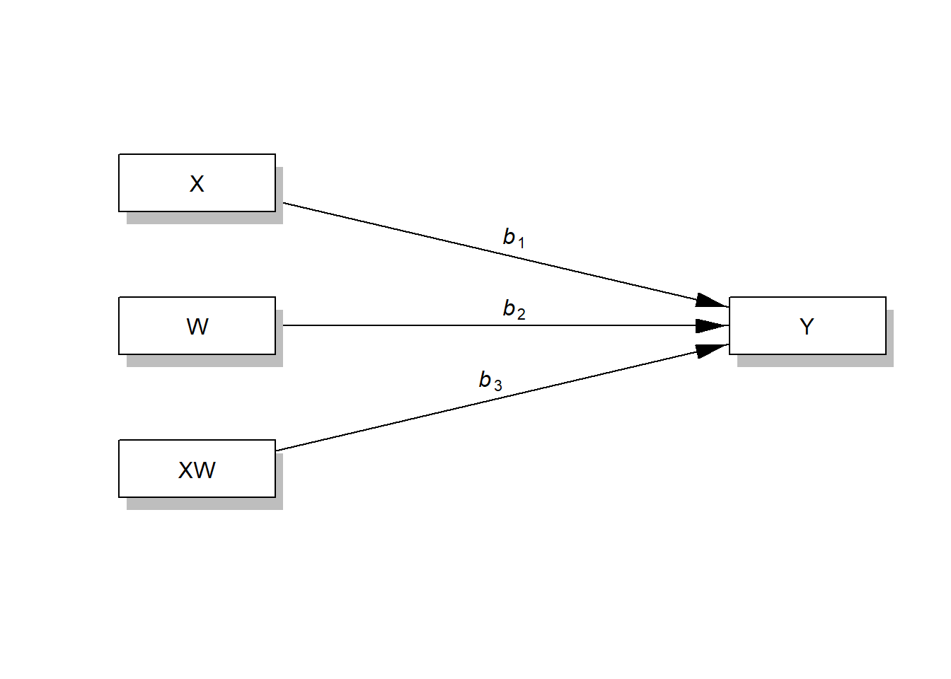
4.3调节模型的实现
## LeaEng~c1*SocMob+c2*PsyCap+c3*SocMob:PsyCap
## PsyCap ~ PsyCap.mean*1
## PsyCap ~~ PsyCap.var*PsyCap
## direct :=c1+c3*PsyCap.mean
## direct.below:=c1+c3*(PsyCap.mean-sqrt(PsyCap.var))
## direct.above:=c1+c3*(PsyCap.mean+sqrt(PsyCap.var))
## lavaan 0.6-3 ended normally after 52 iterations
##
## Optimization method NLMINB
## Number of free parameters 12
##
## Number of observations 895
##
## Estimator GLS
## Model Fit Test Statistic 412.550
## Degrees of freedom 2
## P-value (Chi-square) 0.000
##
## Parameter Estimates:
##
## Information Expected
## Information saturated (h1) model Structured
## Standard Errors Standard
##
## Regressions:
## Estimate Std.Err z-value P(>|z|)
## LeaEng ~
## SocMob (c1) 0.181 1.131 0.160 0.873
## PsyCap (c2) 0.655 0.389 1.684 0.092
## ScMb:PsyC (c3) 0.004 0.016 0.283 0.777
##
## Covariances:
## Estimate Std.Err z-value P(>|z|)
## SocMob ~~
## SocMob:PsyCap 1739.963 92.476 18.815 0.000
##
## Intercepts:
## Estimate Std.Err z-value P(>|z|)
## PsyCap (PsC.) 77.568 0.455 170.565 0.000
## .LeaEng 19.919 32.871 0.606 0.545
## SocMob 24.420 0.190 128.252 0.000
## ScMb:PC 1934.194 22.091 87.557 0.000
##
## Variances:
## Estimate Std.Err z-value P(>|z|)
## PsyCap (PsC.) 14.249 2.428 5.869 0.000
## .LeaEng 148.595 7.028 21.142 0.000
## SocMob 23.077 1.129 20.443 0.000
## ScMb:PC 139721.037 8427.093 16.580 0.000
##
## Defined Parameters:
## Estimate Std.Err z-value P(>|z|)
## direct 0.525 0.122 4.319 0.000
## direct.below 0.509 0.090 5.632 0.000
## direct.above 0.542 0.169 3.216 0.0015.有调节的中介
5.1概念模型
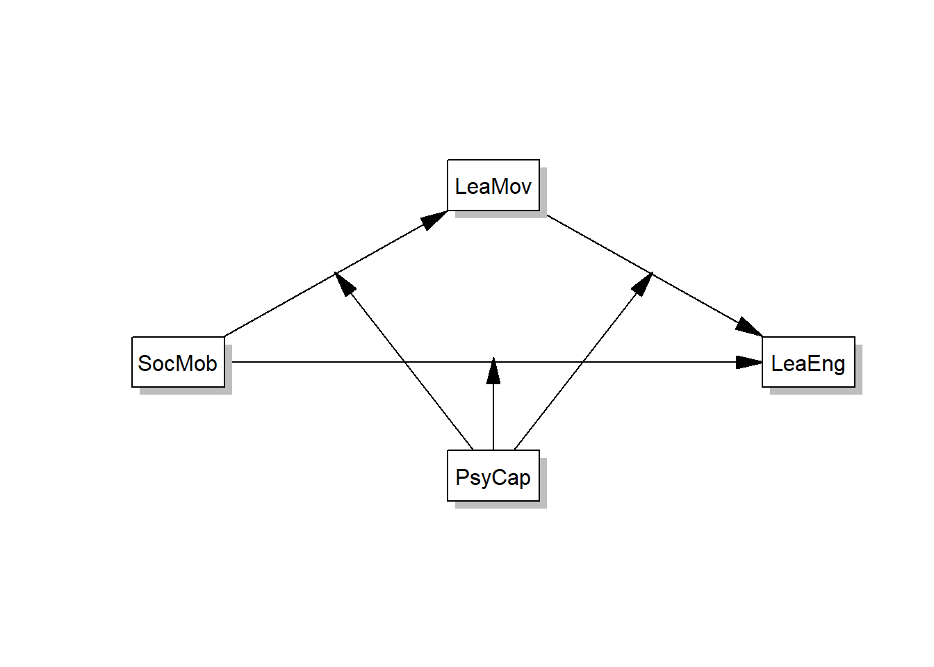
5.2统计模型
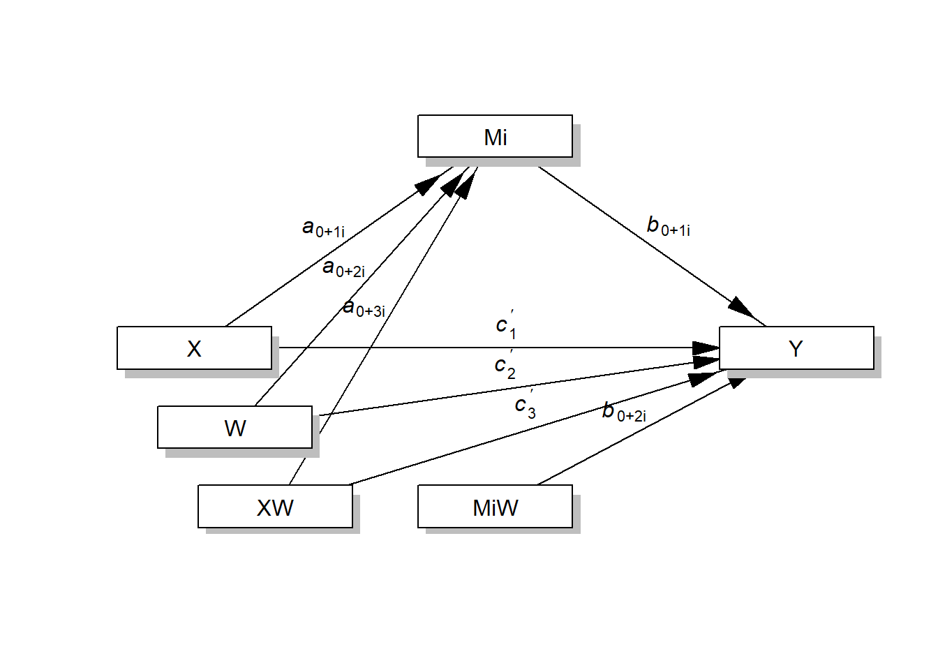
5.3有调节的中介作用模型实现
## LeaMov~a1*SocMob+a2*PsyCap+a3*SocMob:PsyCap
## LeaEng~c1*SocMob+c2*PsyCap+c3*SocMob:PsyCap+b1*LeaMov+b2*LeaMov:PsyCap
## PsyCap ~ PsyCap.mean*1
## PsyCap ~~ PsyCap.var*PsyCap
## CE.XonM :=a1+a3*PsyCap.mean
## CE.MonY :=b1+b2*PsyCap.mean
## indirect :=(a1+a3*PsyCap.mean)*(b1+b2*PsyCap.mean)
## direct :=c1+c3*PsyCap.mean
## total := direct + indirect
## prop.mediated := indirect / total
## CE.XonM.below :=a1+a3*(PsyCap.mean-sqrt(PsyCap.var))
## CE.MonY.below :=b1+b2*(PsyCap.mean-sqrt(PsyCap.var))
## indirect.below :=(a1+a3*(PsyCap.mean-sqrt(PsyCap.var)))*(b1+b2*(PsyCap.mean-sqrt(PsyCap.var)))
## CE.XonM.above :=a1+a3*(PsyCap.mean+sqrt(PsyCap.var))
## CE.MonY.above :=b1+b2*(PsyCap.mean+sqrt(PsyCap.var))
## indirect.above :=(a1+a3*(PsyCap.mean+sqrt(PsyCap.var)))*(b1+b2*(PsyCap.mean+sqrt(PsyCap.var)))
## direct.below:=c1+c3*(PsyCap.mean-sqrt(PsyCap.var))
## direct.above:=c1+c3*(PsyCap.mean+sqrt(PsyCap.var))
## total.below := direct.below + indirect.below
## total.above := direct.above + indirect.above
## prop.mediated.below := indirect.below / total.below
## prop.mediated.above := indirect.above / total.above
## Warning in lav_data_full(data = data, group = group, cluster = cluster, :
## lavaan WARNING: some observed variances are (at least) a factor 1000 times
## larger than others; use varTable(fit) to investigate## Warning in lav_data_full(data = data, group = group, cluster = cluster, : lavaan WARNING: some observed variances are larger than 1000000
## lavaan NOTE: use varTable(fit) to investigate## Warning in lav_model_vcov(lavmodel = lavmodel, lavsamplestats = lavsamplestats, : lavaan WARNING:
## Could not compute standard errors! The information matrix could
## not be inverted. This may be a symptom that the model is not
## identified.## Warning in lav_test_yuan_bentler(lavobject = NULL, lavsamplestats = lavsamplestats, : lavaan WARNING: could not invert information matrix## lavaan 0.6-3 ended normally after 65 iterations
##
## Optimization method NLMINB
## Number of free parameters 23
##
## Number of observations 895
##
## Estimator ML
## Model Fit Test Statistic 4566.675
## Degrees of freedom 4
## P-value (Chi-square) 0.000
##
## Parameter Estimates:
##
## Information Observed
## Observed information based on Hessian
## Standard Errors Robust.huber.white
##
## Regressions:
## Estimate Std.Err z-value P(>|z|)
## LeaMov ~
## SocMob (a1) 0.852 NA
## PsyCap (a2) 0.355 NA
## ScMb:PsyC (a3) -0.005 NA
## LeaEng ~
## SocMob (c1) 1.047 NA
## PsyCap (c2) 0.322 NA
## ScMb:PsyC (c3) -0.008 NA
## LeaMov (b1) -0.410 NA
## LMv:PsyCp (b2) 0.010 NA
##
## Covariances:
## Estimate Std.Err z-value P(>|z|)
## SocMob ~~
## SocMob:PsyCap 3399.918 NA
## LeaMov:PsyCap 3922.738 NA
## SocMob:PsyCap ~~
## LeaMov:PsyCap 637676.532 NA
##
## Intercepts:
## Estimate Std.Err z-value P(>|z|)
## PsyCap (PsC.) 77.568 NA
## .LeaMov 18.366 NA
## .LeaEng 28.295 NA
## SocMob 24.420 NA
## ScMb:PC 1934.194 NA
## LMv:PsC 4469.566 NA
##
## Variances:
## Estimate Std.Err z-value P(>|z|)
## PsyCap (PsC.) 184.686 NA
## .LeaMov 62.424 NA
## .LeaEng 137.790 NA
## SocMob 32.375 NA
## ScMb:PC 435780.850 NA
## LMv:PsC 1586916.422 NA
##
## Defined Parameters:
## Estimate Std.Err z-value P(>|z|)
## CE.XonM 0.454
## CE.MonY 0.364
## indirect 0.165
## direct 0.390
## total 0.555
## prop.mediated 0.298
## CE.XonM.below 0.524
## CE.MonY.below 0.229
## indirect.below 0.120
## CE.XonM.above 0.384
## CE.MonY.above 0.500
## indirect.above 0.192
## direct.below 0.505
## direct.above 0.275
## total.below 0.625
## total.above 0.467
## prop.medtd.blw 0.192
## prop.meditd.bv 0.411